Wall functions and near-wall behaviour
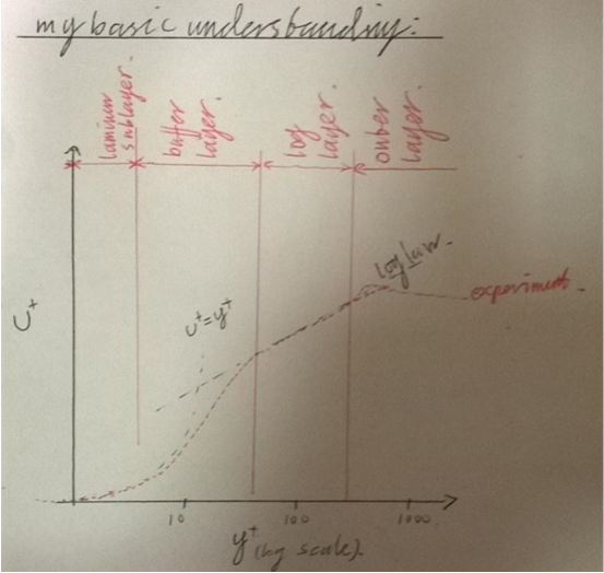
The standard k-e model cannot be integrated down to the wall. (Versteeg and Malalasekera (p77) say that k = 0 and e = 0 at the wall, so eddy viscosity values become indeterminate. Wilcox (p.181) says that when integrated without dampening functions, most turbulence models give false values for C (the additive constant in the log law)).The standard k-e model solves this issue using a wall function. The wall function applies the law of the wall to find the near-wall behaviour. The law of the wall applies to the turbulent boundary layer in scenarios such as pipe flow and flat plate boundary layers. When describing the law of the wall it is generally split into four layers.
The laminar (a.k.a. viscous, linear) sublayer is directly next to the wall. In this layer the velocity profile is linear resembling couette flow. On the wall, the no-slip condition applies and the velocity is zero, outwards from this point the shear stress is roughly constant, and therefore roughly equal to the wall shear stress. u+ = y+ in this region. The real laminar sublayer is very thin (it extends to y = +5 or so).
Between this and the next region is the ‘buffer layer’; The buffer layer is the name for the region between the laminar sublayer and the log-law layer, where experimental data doesn’t quite fit either layers. If it’s to be modelled, it’s usually fitted with a smoothing function.
The next region is the log layer. The velocity profile in the log layer can be described using the law of the wall,  , where
  the Von-Karman constant and C+ = 5 for smooth walls. The log layer extends from about y+ = 30 to y+ = 300, but in some cases (such as turbulent pipe flow) it can give a good approximation of the whole velocity profile.
Beyond this region, the outer layer or “law of the wake” is valid. This region is inertia-dominated core flow far from the wall and free of viscous effects. The law of the wake is:
This is based on the velocity defect law and the names are sometimes used interchangeably.
The aim of the wall function in the standard k-e model is to use these laws to define the velocity in the near wall cell. So the standard wall function uses the log law to define u in the mesh cell nearest the wall, this is why it requires a mesh of between y+ = 30 and y+= 500. So the main advantage of the wall function is that it allows a coarse-grid solution. Measurements of turbulent kinetic energy budgets indicate production equals dissipation. Using these assumptions plus the eddy viscosity formula  the wall function is:
This is applicable at high Reynolds numbers. Fluent contains various variations on this, covered in the theory guide. (I believe ‘scalable wall functions’ <- intended for use with dense meshes, ‘non equilibrium wall functions’ <- a bit of a grey area between the two. Uses log-law with press. grad. correction for velocity & two-layer approach for k)
At low Reynolds numbers the log-law is not valid. Models such as the ‘Low-Re k-e turbulence model’ use wall dampening functions. These can also be referred to as ‘two-layer k-e model’. Fluent calls it ‘enhanced wall treatment’ (Fluent’s ‘enhanced wall treatment’ switches between this and the wall function depending on the y+ of the mesh, using a blending function. The idea is to make the turbulence model robust to coarse mesh regions in the model).
In the theory guide, it defines the enhanced wall treatment as follows. The domain is divided into fully-turbulent and viscosity-affected regions based on wall-distance-turbulent-Reynolds number  is the cutoff point. In the fully-turbulent region, the turbulence model (k-e model or whatever) is solved as per. In the viscosity-affected region, the one-equation Wolfstien (1969) model is used instead, expect for momentum & k, which still follow the k-e model. Turbulent viscosity is found from:
The length scale is found from:
This definition of turbulent visc. is blended with the turbulence model definition (k-e model)
Blending: 
In the viscosity-affected region, turbulent dissipation is found from:  The length scale is found from
  .
.
This is again blended with the bulk values similar to turbulent viscosity above. In simulations where Rey is less than 200 everywhere, e is found algebraically from the above and not from the turbulence model (k-e model or whatever).
For momentum, a blending function is applied. This covers the buffer layer, and allows for including other effects easily (such as pressure gradient effects).
The enhanced wall treatment calculates u+turb as follows, in order to include pressure gradient and heat transfer effects. (I think this and the equation above are all for calculating u in the first cell only? i.e. this is how it switches between a wall function approach and a low-Re approach?):
Solving the above is an ODE that Fluent solves analytically. If all three constants equal zero, then this becomes the log-law. For u+lam:
(the manual then covers a thermal boundary layer equation, which I will leave out).
(I think there’s two issues going on: I think wall dampening functions are needed to control turbulence values (k etc) near to the wall, but a value for the boundary condition (the first cell) also needs to be defined.? )
Trying to shed some light on the k-w model behaviour in the near-wall region:
Quotes on k-ω:
Versteeg and malalasekera, p 91:
“the k-ω model initially attracted attention because integration to the wall did not require wall dampening functions in low Reynolds number applications”
Not the most academic reference! forum post:
“the k-omega based models were designed originally for the near wall region and therefore does not require dampening functions, hence hybrid wall functions (blending of near wall and log law function) were implemented directly and same is true for SA model”
Ansys Fluent theory Guide, p114, p 126:
“y+ independent formulations are the default for all ω-equation based turbulence models… …for the ω-equation based models, use the default – EWT(enhanced wall treatment)- ω … (p126) EWT-ω: Unlike the standard ε-equation, the ω-equation can be integrated through the viscous sublayer without the need for a two-layer approach…”
CFD online Wiki:
“the SST k- ω model can be used as a low-Re turbulence model without any damping functions”
(Section afterwards says fluent uses wall functions unless “transitional flows option” is enabled. I think the author could be getting “transition-SST” and “Low-Re” options in Fluent confused ?)
Wilcox, p 181:
“the k-ω model is, in fact, unique because viscous modifications to its closure coefficients are not needed to achieve a satisfactory value of C”
(does not mean that corrections are not used at all !!)
Boundary conditions, SST k-w Model, Fluent Theory guide:
For the k-w model at the wall boundary condition, a switching function (not given in fluent guide, CFD online suggest route-mean-square type belnding function) blends between these two values depending on the grid density.
According to Versteeg and Malalasekera (p 91), this is the hyperbolic variation of w at the near-wall grid point. it is more commonly seen as  elsewhere. Fluent’s equation looks different but is actually the same if you do the algebra subbing in the dimensionless no’s.
Boundary condition for k are “as for enhanced-wall treatment” in the k-e model. Not really clear what this is in actuality. Closest is page 118 in Fluent theory guide:
where ‘n’ = local coordinate relative to cell wall. Versteeg and Malalasekera state “k at the wall is set to zero” for the k-w model. This stems from the no-slip condition, according to Wilcox (p.176).
k = 0 and ω as table supported by NASA website. also gives “farfield values” (I think this is recommended inlet & outlet conditions?)
low-Re SST in fluent theory guide:
The low-Re correction is nothing to do with the transition-SST model. The low-Re correction acts on μt and is available in the k-ω models:
Sources:
Versteeg, HK. Malalasekera, W. (2007) An introduction to computational fluid dynamics. 2nd ed. Prentice-hall.
Wilcox, DC. (2006). turbulence modelling for CFD. 3rd ed. DCW industries.
Wolfstien (1969). The velocity and temperature distribution in one-dimensional flow with turbulence augmentation and pressure gradient. International journal of heat and mass trans 12(3). can’t access requires ILL?
NASA website: https://turbmodels.larc.nasa.gov/sst.html