Including a diameter-dependent Cunningham slip correction factor in Fluent.

Very small particles (typically < 1 micron) do not obey Stokes law for drag when they are suspended in a gas. The particles are so small that they experience interactions with the gas not as a continuum, but as individual collisions. The main outcome of this is that the assumption of a no-slip boundary on the particle’s surface is no longer true. Small particles have less drag than is calculated by Stokes law, and this can be corrected for using Cunningham slip correction factor.

The Cunningham slip correction factor can be set in Fluent when defining the injection. So, say you have a particle injection of 0.1um diameter, you can set the drag law to “Stokes-Cunningham” and add the Cunningham slip correction factor as a constant (say “11.0”) that is relevant to the size of that particle.

But what if you’re particle is changing in size as it moves through the domain ? What if you particle is growing through condensation, or losing mass through evaporation ? What if you inject a distribution of particle sizes rather than just one size ? In these cases, the particle will have a diameter-dependent Cunningham slip correction factor – it won’t be just one value.

There’s no option to support this in fluent, so I have wrote a quick UDF that deals with it. I have tried to stick to the Fluent defaults as much as possible. To calculate the drag, I’ve used the same source as Fluent for it’s default, “spherical” drag law (Morsi and Alexander, 1972). To calculate the Cunningham Slip correction factor, I’ve used the formula given in the Fluent Theory Guide (page 386, eqn 16.69). it’s worth noting here that the constants used in the Cunningham correction formula here are for air, if you’re looking at a different gas you’ll need different constants (see the Wikipedia article: https://en.wikipedia.org/wiki/Cunningham_correction_factor). I’ve used the mean free path formula for air, taken from Flaggan and Sienfield (2012, p. 296) and added the values that are constants assuming a pressure of 1atm:

equation 1: mean free path of air

Fluent’s receives the drag force in the form of the dimensionless group 18*Cd*Re/24. So as you’ll see below the drag force is converted to this before it is returned to Fluent, and the Cunningham correction is also applied as appropriate.

Here is the resulting UDF, which must be “complied” and must be “hooked” as described in the Fluent UDF manual for Define_dpm_drag. Please feel free to use my code, as long as you reference my blog.

/*the following implements a diameter-dependent Cunningham slip correction factor*/

/*Actual drag coeffs used by Fluent have been referenced-chased (Morsi, SA. Alexander, AJ. (1972). An investigation of particle trajectories in two-phase flow systems)*/

/*CFDYouself.blogspot.co.uk, JRH, 09.10.15 */

#include "udf.h"

#include "math.h"

DEFINE_DPM_DRAG(cunningham_drag_force, Re, p)

{

cell_t c = P_CELL(p);

Thread *t = P_CELL_THREAD(p);

real lambda;

lambda = 0.0002135166*C_MU_L(c, t)*sqrt(C_T(c, t));

real Cc;

Cc = 1 + (2 * lambda / P_DIAM(p))*(1.257 + 0.4*exp(-1.1*P_DIAM(p) / (2 * lambda)));

real Cd, drag_force;

if (Re < 0.1)

{

Cd = 24 / Re;

drag_force = 18*Cd*Re/(24*Cc);

return (drag_force);

}

else if (Re < 1)

{

Cd = 22.73 / Re + 0.0903 / (Re*Re) + 3.69;

drag_force = 18 * Cd*Re / (24*Cc);

return (drag_force);

}

else if (Re < 10)

{

Cd = 29.1667 / Re - 3.8889 / (Re*Re) + 1.222;

drag_force = 18 * Cd*Re / (24*Cc);

return (drag_force);

}

else /*if (R < 100)*/

{

Cd = 46.5 / Re - 116.67 / (Re*Re) + 1.6167;

drag_force = 18 * Cd*Re / (24*Cc);

return (drag_force);

}

/*included incase needed later - not needed here.

else if (Re < 1000)

{

Cd = 98.33 / Re - 2778 / (Re*Re) + 0.3644;

drag_force = 18 * Cd*Re / 24;

return (drag_force);

}

else if (Re < 5000)

{

Cd = 148.62 / Re - 4.75e+4 / (Re*Re) + 0.357;

drag_force = 18 * Cd*Re / 24;

return (drag_force);

}

else if (Re < 10000)

{

Cd =  -490.546/ Re - 5.79e+5 / (Re*Re) + 0.46;

drag_force = 18 * Cd*Re / 24;

return (drag_force);

}

else

{

Cd =  -1662.5/ Re - 5.42e+6 / (Re*Re) + 0.5191;

drag_force = 18 * Cd*Re / 24;

return (drag_force);

} */

}

Morsi, SA. Alexander, AJ. (1972). An investigation of particle trajectories in two-phase flow systems. Journal of Fluid Mechanics, 55(2), pp 193-208.

Ansys, (2013). Ansys fluent theory guide release 15.0. Canonsburg: Ansys inc.

Flaggan, R. and Sienfield, J. (2012) Fundamentals of air pollution engineering. Mineloa: Dover Publications.

Correction for Heterogeneous Nucleation

heterogeneous nucleation

Frequently studies which use classical nucleation theory account for heterogeneous nucleation using a heterogeneous nucleation correction factor. This is normally denoted f(θ) or something similar, and is inserted into the classical (homogeneous) nucleation rate equation to account for the effect of nucleation on a surface. In this blog entry I’m going to cover this factor. The “flat surface” correction is common because in most of the cases commonly studied the foreign nuclei is much larger than the critical cluster that is forming on its surface, so the contact surface between them can be considered flat. A more complicated version of f(θ) can be derived for a curved foreign nucleus, derivation is covered in Vehkamaki (2006) ch. 7. This subject is something of a departure from the normal subjects discussed on this blog, as this correction to my knowledge is not available in default settings of any particle formation laws etc. in Fluent (Fluent is the software I currently use exclusively for CFD). But It’s still of interest to the particle formation stuff I’m working on currently. 

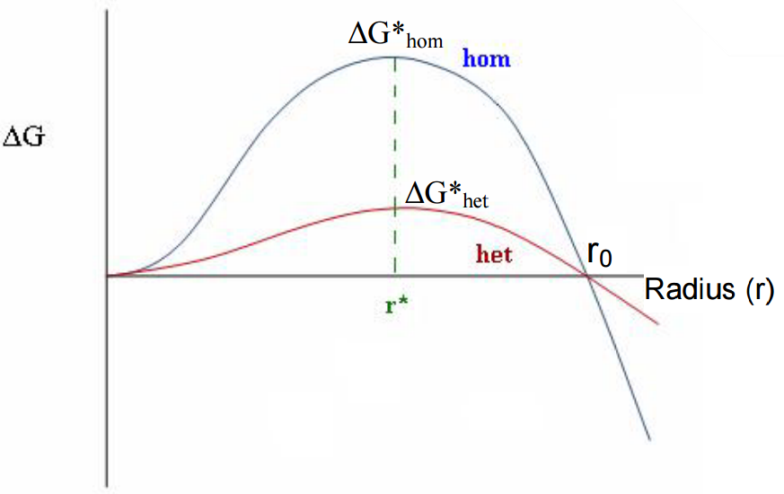
Heterogeneous nucleation has an effect that is similar to catalysis in reactions. It lowers the energy barrier. Heterogeneous nucleation happens faster at lower degrees of supersaturation due to this change in the critical Gibbs free energy.

Figure 1 – A graph showing the effect of heterogeneous nucleation on critical energy (Zang, 2015).

The correction factor was originally derived by Fletcher in 1958, and is sometimes referred to as the “Fletcher factor” (Kalikmanov, VI. 2013). But Equation 1 reduces to the flat-surface correction when the curved surface is very large.

 

Equation 1 – The long-winded version of Fletcher factor, for curved surfaces. Dimensionless versions are common. Here a is the ratio between the foreign nucleus and the cluster; m is the cos of the (cluster) contact angle; w = √1+a2-2ma.

The flat surface correction is:

Equation 2 – The flat-surface correction. υ is the contact angle (between the critical droplet on the surface).

For the heterogeneously nucleating critical droplet, the radius is exactly the same as for the homogeneous case, but the volume of the nucleating particle changes because the particle becomes a spherical cap instead of a sphere. Equation 2 corrects for this reduced volume (which reduces the critical Gibbs free energy, the critical Gibbs free energy is the point where the (-ve) volume free energy change balances the (+) free energy change needed to create a surface). The angle can be found by young’s equation if the surface tensions between the gas, cluster and substrate are known.

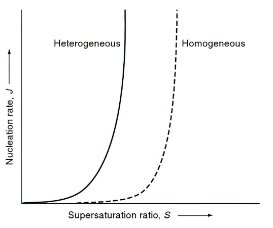
Figure 2 - Effect of heterogeneous nucleation on the nucleation rate. shamelessly copied-and-pasted from Coulson 2.

How it is applied in the nucleation rate equation (shown in Equation 3). The biggest difference comes in the form of the effect on ΔG*het. Typically the pre-exponential factor may be known experimentally (typical value is around 1017 cm-2s-1 for heterogeneous vapour condensation). The monomer flux (W*) is the sum of both the molecular-bombardment style growth present in homogeneous nucleation (R* = monomer flux, s* = surface area of critical droplet) but also adatom impingement (W*s) – surface diffusion of adsorbed atoms to the nucleus periphery.

Equation 3 - Difference between heterogeneous and homogeneous nucleation, (Cooper, 2015).

Most sources simply state that the dependency of Jhet on the corrected free energy, and do not discuss the pre-exponential factor in detail. However, Fletcher (1959) himself states that heterogeneous nucleation requires changes to this pre-exponential factor (though he does not cover what these changes are in the source). Talanquer and Oxtoby (1996) give an example of an analytical expression for this pre-exponential factor in their paper. However, overall this is all there is to the classical treatment of heterogeneous nucleation.

Cooper, S. (2015). Crystallisation Kinetics. Durham University. Available: http://community.dur.ac.uk/sharon.cooper/lectures/cryskinetics/handoutsalla.html accessed: 17 Aug 2015.

Fletcher, NH. (1959). On ice-crystal production by aerosol particles. Journal of Meteorology. 16(2). pp. 173-180.

Kalikmanov, VI. (2013). Nucleation theory. Berlin: Springer.

Vehkamaki, H. (2006). Classical nucleation theory in multicomponent systems. Berlin: Springer.

Zang, L. (2015). Lecture 12 Heterogeneous Nucleation: a surface catalysed process. College of engineering University of Utah. Available: http://www.eng.utah.edu/~lzang/ accessed: 12 Aug 2015.

Kantrowitz Factor

Kantowitz Factor

Kantowitz factor, (often simply called the non-isothermal correction factor), is applied as a correction to the nucleation rate from classical nucleation theory. In most cases (the example here is taken from the wet steam model chapter of the fluent theory guide) it appears as follows:

Equation 1 –typical nucleation rate given by Classical Nucleation Theory, with Kantowitz factor 1/1+θ up front.

The non-isothermal factor is found from the enthalpy and the ratio of specific heat capacities:

Equation 2 – non isothermal correction factor.

According to Bakhtar et al (2005) this is a simplification that can be made at low pressure, when the critical radius is much smaller than the mean free path of the gas. Really it should look like:

Equation 3 – nonitsothermal correction factor is a simplification of this.

In the presence of a large volumes of inert gas, isothermal assumptions are justified because collisions with the inert gas, (which transfer heat) are much more common than those with condensing species.

The derviation of the Kantrowitz factor (and Feder’s correction factor) assume that every cluster is at the same elevated temperature. Wyslouzil and Sienfield (1992) criticise this, on the basis that the temperature of small (subcritical) clusters is more sensitive to the addition of more molecules, and the growth of these small clusters affects the final result.

Feder also came up with their own correction factor of the form shown below, that is used in a similar way to the Kantrowtiz factor.

Equation 3 – feder's factor - similar to 1/1+θ .

It results is around 0.01 or a hundredth of the isothermal (Wu, 1973), though it’s worth mentioning that most of these flows are very fast – discussions in the literature centre exclusively on nozzles and steam turbines. b and q are defined in terms of thermodynamic state of the supersaturated vapour. q is basically mostly latent heat. The b is calculated from β, gas kinetic collision frequency (Dawson et al. 1969).

Pandey 

Equation 3 – feder's factor - nuts and bolts.

(2014, p. 15) discusses the steady-state assumption in connection to the Kantrowitz factor. τ = 10-7 to 10-6 s is the timescale for ‘steady state nucleation rate’. Cooling rate ranges from 0.2-0.8 K/µs. The characteristic time in nozzle flows is typically τ = 10-3 s. Kantrowitz factor uses a steady-state assumption, so it is justified on this basis, for use even for unsteady state assumptions.

So to conclude on Kantrowitz factor, corrects for non-isothermal effects which make the nucleation rate about 50 to 100 times slower in rapidly expanding steam flows, such as steam turbines and nozzles. It assumes a steady-state conditions but this is valid as the time to reach steady state is so small. However, it’s the problem of non-isothermal particles itself is less of a big deal when the bulk of the gas is an inert component (such as air) – in these cases the inert gas collisions conduct heat much faster than the particle can grow. Also, my brief lit review hasn’t shown a Kantrowitz factor being applied to something that isn’t a turbine or a nozzle. Feder’s factor is used an alternative, but is basically for similar purposes.

Bakhtar, F. et al. 2004. Classical nucleation theory and its application to condensing steam flow calculations. Proceedings of the IMechE, 219 C. p. 1315-1333.

Pander, A (2014). Numerical modelling of non-equilibrium condensing steam flows. Delft University.

Wu, B. 1973. Possible condensation in rocket exhaust plumes 2. Yale University.

Wyslouzil, BE. Sienfield, JH. 1992. Nonisotermal homogeneous nucleation, 97 (4). pp. 2661-2670.

Thermophoresis

Small particles in suspension are subject to forces caused by random collisions with gas molecules. Brownian motion for example, is an observable effect of these random collisions.

A suspended particle in a temperature gradient experiences a force known as thermophoresis. Hot gas molecules collide with one side of the particle on average with greater force than cold gas molecules collide with the opposite side. This creates a net force on the particle towards the cold gas region and away from the hot (Bott, 1995).

This effect can be exploited in industrial gas cleaning operations, in the form of a ‘thermoprecipitator’ or ‘thermopositor’. Like an electrostatic precipitator, thermophoresis creates a force on the particle towards a cold surface, eventually the particles collide with and deposit on the surface (Davis and Schweiger, 2002).

Ansys Fluent allows the user to include thermophoretic force on particles in DPM simulations, through a tickbox option in the GUI. A closer look at the Fluent Theory Guide shows this is (unless otherwise specified by the user) calculated using an equation from Talbot:

Equation: Talbot equation for thermophoretic force. Where: dp = particle diameter; µ = fluid viscosity; Cs = 1.17; K = k/kp (k = fluid thermal conductivity based on translational energy only k = 15/4 µR; kp = particle thermal conductivity); Cm =1.14; Ct = 2.18; Kn = Knudsen number = 2λ/dp; λ = mean free path of fluid; mp = particle mass. The equation assumes a spherical particle & ideal gas behaviour.

The referenced paper by Talbot (1981) consists of a comprehensive literature review with some experimental work. This expression is actually attributed to JR Brock, and Talbot simply suggests adjustments to the C constants. Division by mp is due to the fact Fluent accepts F in units of acceleration not force.

Talbot explains that this equation is theoretically applicable for Kn < 0.1 as this is the limit of the Basset drag formula that forms part of Brock’s derivation. But Talbot also shows the expression (with the revised constants) reduces to the Waldmann formula for Kn tending to infinity. In the appendix Talbot also provides a rough discussion of the applicability of the formula in the intermediate range of Kn.

Bott, TR. (1995). Fouling of Heat exchangers. Amsterdam: Elsevier. pp.67  

Davis, J. Schweiger, G. (2002). The Airborne Microparticle. Berlin: Springer. pp. 756

Talbot, L. et al. (1981). Thermophoresis of Particles in a Heated Boundary Layer. Journal of Fluid Mechanics. 101(4). pp737-758.  

Possible options for modelling particulate formation in Ansys FLUENT

The following is just a quick going over of some options I’ve come across so far for modelling
particulate-formation type behaviour in Ansys Fluent. The list is by no means exhaustive. Most of this information is summarised from ansys literature.

Discrete Particle Modelling

- I could use literature data to find the concentration and particle size of contaminants
normally present in air that drive heterogeneous nucleation. I could use
this to set up the injection of DPM particles
- I could then define the particle diameter as a variable, and define the growth rate based on:
(size, temperature, partial pressure, mass transfer film resistance) using UDFs.
Advantages:
- Already working with discrete particles; continuation of a theme.
Disadvantages:
- Contaminant concentration is a guess.
- Does not account for transfer to the walls.
- UDFs more complex than they sound: growth will require source terms, will still require a  multispecies gas phase,
- I haven’t found a tutorial that covers condensation using DPM. The options for heat & mass
transfer in DPM are “Droplet (heating, evaporation, boiling)”, “Multi-component
(multicomponent evaporation), “Combusting (Heating, de-volatilisation, heterogenous
reaction)”. Condensation is not included in Fluent, and a User Defined Function is required.

Evaporation-Condensation Modelling:

Is available with mixture models and Eulerian multiphase. Option of Lee model or the Thermal Phase Change model.

Lee Model:

The theory guide mentions the Hertz-Knudsen equation. This equation is re-arranged so that the

driving force is defined based on Tsat rather than Psat.  The following coefficient is a constant in the

model defined by the user:

mass trans. is defined:    

Nb. These equations are for evaporation, but condensation equations are of the same form.
The user guide states “diameter (dh) and accommodation coefficient (B) are usually not very well known, which is why the coefficienct “coeff” must be tuned to experimental data”. Personally, I think this could be problematic because we expect that dh and Tsat change with condensation properties. In this model the user defines “coeff” as a constant and I don’t think it can be defined as a UDF. This model is capable of defining the saturation temperature in terms of total pressure, but it requires  a UDF to define saturation temperature in terms of partial pressure.
Advantages:
- Looks simple to implement. Based on a tutorial I tried modelling condensation of pure steam
at ~+100degC and it seemed to give OK results.
Disadvantages:
- Over simplistic, assuming “coeff” and “dh” are const. for condensation from an inert gas like air, we also need saturation as a function of partial pressure.

Thermal Phase Change Model:

Thermal phase change model uses the two resistance model to model heat transfer (which is basically h-values for liquid & vapour phase heat transfer coefficients). The mass transfer is the governed entirely based on the heat transfer process and the overall heat balance. Only works with a Eulerian model.  In this model you specify (along with the heat transfer characteristics) the continuous phase and dispersed phase transfer coefficients. According to the user guide these “act as multipliers for the heat transfer coefficients determined for each phase and the default value of 1 is usually appropriate”. This factor doesn’t seem to appear in the equations in the theory guide.

Advantages:
- Some of the literature I have read actually states growth of particles can be heat-transfer limited.
- Seems more appropriate than the Lee model at face value.
Disadvantages:
- Would still require a UDF for saturation in terms of partial pressure.

Soot models:

Three soot models exist in Ansys.
1. One-step model (Khan and Greeves), single transport eqn. for soot mass fr.
2. Two-step model (Tesner) transport eqns for radical nuclei concentration and soot mass fr.
Both models use empirical rate constants for soot formation.
3. Moss-Brookes model, solve transport eqns for soot mass fr. And normalized number density.
Moss-Brookes Hall model – as above for hydrocarbons larger than methane.

In Khan and Reeves model the source term takes a form similar to the Arrhenius equation. You can define the formation const. Cs, the equivalence ratio exponent r, activation temperature E/R. In the Two-step model, nucleation is defined using a simpler Arrhenius-type equation with branching and collision terms included. The rate of soot formation depends on the nucleation rate, but it also involves two empirical constants. The mean particle size is predefined, so this model isn’t actually modelling particle growth. In the Moss-Brookes model the nucleation is dN/dt, the source term for the number density. The mean diameter in this model is used to find the coagulation rate. But dM/dt has a surface growth term – this is the source term in the soot mass fraction equation. So (I’m guessing) if N & M both change separately, then you know the number and you know the mass fraction of particles, so you can work out what the mean particle size must be from these two
values.

Advantages:
- The soot models are built into fluent. Could be faster or easier than writing UDFs

Disadvantages:
- All of the models are highly empirical and application specific to soot formation.
- Adjusting the model parameters might eventually lead to something representative of
another particulate formation in another scenario, but these parameters must be set as
constants and cannot be UDFs, which could be restrictive.
- Possibly wrong tool for the job.

Eulerian wall film:

Eulerian wall film model is relevant as it can be used to model particle capture & inclusion into films. It can model film condensation and evaporation, as well as ice accreditation on aircraft. Can model heat & mass transfer in evaporation & condensation. Solidification, Melting & sublimation possible
through UDFs. Works with DPM and Euler-Euler particle models. The wall film is transient, but it can be used in steady-state flows with the “film time step size”. Using the wall film model with mixture species transport allows us to model mass transfer from an inert gas using partial pressure.

Population Balance Modelling: 

Population Balance Modelling applies to Eulerian multiphase models. Nucleation can be specified as constant, or via a UDF. There are five types of population balance model, in two categories:

1. Discrete method:
a. Homogenous discrete
b. Inhomogenous discrete
2. Method of Moments:
a. Standard Method of Moments
b. Quadrature Method of Moments
c. Discrete Quadrature Method of Moments

The Discrete, homogenous model uses Hounslow’s approach for bin discretisation, which uses geometrically increasing bin sizes. Homogenous models have only two phases. Particles share velocities, so it won't model segregation of larger particles by settling or impaction. In the discrete inhomogeneous model the bin sizes are at the discretion of the user. Each bin size is handled as a separate phase, so the computational load is higher, but each bin has its own velocity allowing size separation to be modelled.The method of moments uses the moments of the distribution in place of the distribution itself. The resulting distribution can then be reconstructed from the moments to give the “statistically most probable distribution”. The quadrate method of moments allows breakup & coalescence to be modelled, but similarly to the standard method, describes every particle with a single velocity field. Discrete quadrature method of moments allows for different velocity fields on different particle sizes, nucleation and growth modelling in population balance models.Nucleation is defined as a boundary condition, in the discrete methods, it creates particles at a constant rate in the smallest size bin. Nucleation rate can be defined as a constant or as a UDF. Growth rate in m/s can also be defined as constant or via a UDF. Neither of these are available when using inhomogeneous discrete method. For the Standard method of moments, only size-independent growth is available. You can add mass transfer using species transport options. You have the choice of: none, constant rate, user defined, population balance. In the latter nucleation and growth rates are calculated by the population balance kernels.

2334 5367 .2/ 0 1 58