Discretisation in Fluent

Fluent has a variety of options for the solver. In this post I’ll be covering first and second order upwind schemes. Other options exist, such as QUICK and MUSCL, but I will leave these out. I’ll also be concentrating on pressure based solver, solving at the cell centres, in steady state simulations (laminar & RANS).  

Most CFD uses a finite volume method to discretise the PDEs. The PDEs are integrated, and this puts them in a form that applies to a single mesh cell.

Becomes,

.

The integration over the cell faces (integral with circle through it) comes from the “divergence theorem”. The resulting sums balance flows into and out of the cell (Craft, 2011). The transient term (∂ρφ/∂t V) is defined by the temporal discretisation and equals zero in steady state.

As the flow is actually being solved, the value of the variable at the current cell centre and the cell face, φ and φf, are unknown. Generally, the value in the current cell is expressed in terms of the faces values, and the face values are found from the cell-centred values in surrounding cells. This gives us a linearized set of equations of the form:

The a’s are the ‘linearised coefficients’, subscript p refers to current cell, nb refers to neighbouring cells. An example is included below in Figure 1 for the first order upwind case. The coefficients anb and b will be different for every cell in the domain, at every iteration. The field for φ can be calculated by recalculating iteratively for all of the cells in the domain.

Most of the interpolation schemes focus on how the face value φf can be calculated from the neighbouring cell values. For the first order upwind scheme, face value φf is equal to the upstream cell-centre value.

---

---

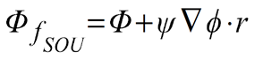
For the Second order upwind scheme:

In the equation immediately above, φ and nabla φ are found in the upstream cell. “r” is the displacement distance from the upwind cell centre to the cell face. This is the main difference between first and second order upwind methods: instead of assuming the value of φ is constant over the upstream cell, the second order upwind scheme basically uses ‘linear interpolation’ (in a loose sense) of the gradient (nabla φ) in the upstream cell to find the values at the face.

nabla φ itself found through a “least-squares cell-based” method by default in fluent. (in basic terms, a sort of ‘weighted average’ of the surrounding cell values is used to find the gradient in each cell).

The theory guide mentions a “Multi-dimensional linear reconstruction approach”, and references Barth & Jespersen (1989).  I have taken this out on interlibrary loan, but reading the paper hasn’t significantly improved my understanding of the second order upwind scheme. My understanding of what they mean by “multi-dimensional linear reconstruction” is just what has been described – you find the cell-face value using the gradient.

Gradient Limiters:

This isn’t the end of the story because the second order upwind method can create spurious oscillations. The calculated cell face value has to be between the values of the two cells (current cell centre and the upwind cell centre) to prevent spurious oscillations. This is the monotonicity principle and is applied in Fluent through Gradient limiters. These are typically applied as shown (ψ = gradient limiter).

There are three different types in Fluent:

• Standard limiter
• Multidimensional limiter
• Differentiable limiter

Ψ is a factor between 1 and 0, so ψ = 1 is fully 2nd order upwind, ψ = 0 is fully 1st order upwind (φf = φupstream cell). In the standard limiter, ψ is calculated to force φf to be between the min & max of the neighbouring cells*. In the standard limiter a minimum ψ is found in each cell and applied to every face, while the multidimensional limiter applies a different ψ to each face of the cell. Differentiable limiter is more complex & perhaps appropriate for a later blog entry.

References:

Craft, TJ. 2011. Review of Basic Finite volume Methods. (Unpublished) University of Manchester.

Bakker, A. 2002. Applied Computational Fluid Dynamics Lecture 5 – Solution methods. (unpublished) www.bakker.org accessed 20th January 2016.

Barth, TJ. Jespersen, DC. 1989. The design and application of upwind schemes on unstructured meshes. 27th AIAA meeting,

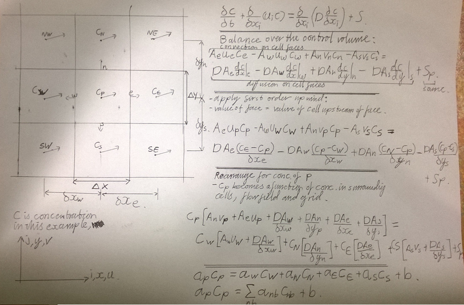
Figure 1 - Example of the discretisation process, for a first order upwind scheme (Bakker, A. 2002)

*by “neighbouring cells” we mean the minimum or maximum of the cell centre values of all the neighbour cells of the upstream cells. This is covered in Barth & Jespersen (1989)

Euler-Lagrange models (DPM)

Below are some eclectic notes on DPM I thought would be worth uploading. The section begins with DPM basics and goes on to discuss stiff DPM type problems. Please excuse the non-standard referencing and abruptness. the bulk of this info is simply re-constituted from the Ansys literature. The 2nd half of the post looks briefly at how heat transfer is modelled for the particles.

Source: http://www3.nd.edu/~gtryggva/CFD-Course2010/2010-Lecture-19.pdf

The most important equation for Euler-Lagrange models is:

The force balance is usually something like this:

Drag + gravity & buoyancy + other forces (lift, added mass, pressure… thermophoresis?)

When the effect of the particles on the fluid is not considered, this is known as one-way coupling. The DPM source terms are not included in the flow calculations, and DPM is applied as a post-processing technique.

When the effect of the particles on the fluid is considered, this is known as two-way coupling. The DPM source terms are included in the flow calculations. In this case, the particles need to be iterated with the flow. The DPM underrelaxation factor defines how many iterations are required for the source terms to take full effect on the flow. This is described by the graph below, you can see the default DPM URF = 0.5 takes about 10 iterations to update the source term, 10 iterations is the default setting for the “number of continuous phase iterations per DPM iteration” in Fluent.

• Source: ansys fluent lectures – combustion 14.0 – dpm. Best practice for DPM reactive flows

The default URFs are fine for simple cases. For more complex cases default URF can be too aggressive. Effect of URF is highly non-linear. You can increase the number of stochastic tries for turbulence random walk models in order to even out the particle’s effect on the flow. Underrelax the species and energy to start-up the solution (recommends 0.9 for each) then once solution is stable, attempt to increase these to 1.

Source: fluent lectures – combustion 15.0_L4_DPM.

Often the convergence problem is related to high source terms generated in certain cells. Try increasing stochastic tries, and increase the number of gas-phase iterations per DPM iteration. Energy, radiation and ‘mixture fraction’ (species) should have residuals less than e-6.

Node based averaging spreads the load of a DPM source into neighbouring cells. Good for reducing grid dependency, and improving convergence in steady-state sims. “Enable Node-Based Averaging”.

Source term linearization can be combined with node based averaging for simulations without mass transfer. Must be done with caution - see below.

Source: Ansys Fluent lectures – multiphase -15.0 – DPM.

Solution strategies for steady flows in DPM

1. Closer coupling between the dispersed and continuous flow.
1. Increase underrelaxation factor for discrete phase
2. Decrease number of continuous phase calculations between trajectory calculations
3. Lower the underrelaxation factors for the continuous phase
2. Decoupling between dispersed and continuous flow.
1. Lower the underrelaxation factor for discrete phase
2. Increase number of continuous phase calculations between trajectory calculations

_____________________________________________________________

DPM Switching Laws

When modelling droplet evaporation, it is advised to always inject particles at a temperature a few degrees below their vaporisation temperature in order to improve stability.

When modelling heat transfer in DPM, irrespective of inert, droplet, or multicomponent particles, DPM switching laws are active. an example of switching laws progressing for a combusting particle:, in order of increasing temperature of particle

1. inert heating law
2. drying (water removal) - (evap, boil, inert heating)
3. ...
4. devolatilisation
5. combustion
6. inert heating

Inert heating or cooling: Law one, Law six.

Law one: apply when the particle temperature is less than the defined vaporisation temperature.

Tp < Tvap.

Law six: apply when the volatile fraction fv0 of the particle has been consumed (think this applies to coal combustion models etc). “Equation is saying: activate inert heating when the particle mass has dropped to that of the non-volatiles only”.

The “Inert Heating Law” is a simple single-film equation, with radiation heat transfer added-on.

,h = convective heat transfer coefficient. W/m2. Found by Ranz-Marshall correlation.

Droplet Vaporisation: Law Two

Applies between the vaporisation temperature and boiling pt temperature (or until the volatiles are completely gone).

The “diffusion controlled model” is just a single-film mass transfer law, which assumes the particle Temperature = equilibrium vapour concentration at the particle surface, and that raoult’s law applies in the bulk. Mass transfer resistance is found using the “Sherwood number correlation” which is just the Ranz-Marshall correlation with Heat/Mass Transfer Analogy applied (the one where you just replace dimensionless numbers).

Defining boiling point and latent heat

This is a Hess’s law-style enthalpy balance to extrapolate the latent heat at the boiling down to the vaporisation temperature. This is only active when “temperature dependent latent heat” is selected in the discrete phase model dialogue box.

• (P-1 or DO, radiation modelling) when Radiation modelling is OFF, therefore the problem can’t be anything to do with radiation terms.
• “temperature dependent latent heat” is off, therefore the problem can’t be anything to do with hess’s law-style calc.

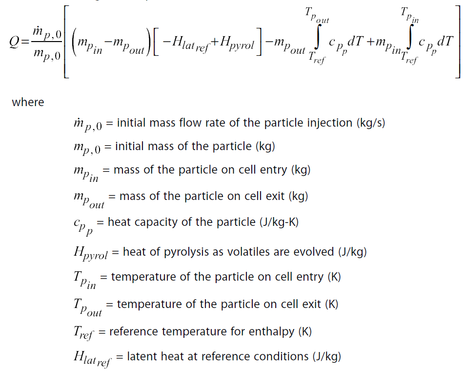
Enthalpy balance for DPM source: P 494, Ansys theory guide

____________________________________________________

Linearize source terms: this option linearizes DPM source terms for momentum, energy and species w.r.t. cell variable φ. SDPM = Sconst  + Slin φ . Increases numerical stability for steady flows. Transient flows => longer time steps and larger URFs (+ve).

Have to be careful when used in conjunction with average DPM source terms, combining the two for vapourising particles can lead to numerical instabilities and unphysical results for gas temperature.

First to Higher Order Blending

This is just a quick post on first-to-higher-order blending. First-to-higher-order blending is used when you want something in between a first order upwind and a second order upwind scheme in your simulation. Say you are trying to solve, and you get good convergence in first order, but when you move to second order you have trouble getting a converged solution - you can use first-to-higher-order blending to make this change gradually.

I've written a scheme journal file that'll do this gradual ramp-up. Scheme can be used just like a normal journal file. I've found the main difference between scheme and journal files is that scheme code gives you more options. Here I'm using scheme to do a loop (which to my knowledge isn't possible in an ordinary journal file). I've found that one downside is that scheme is more difficult to cancel & quit halfway through a calculation. It can also be more difficult to write.  

This scheme file slowly ramps up the first-to-higher-order blending value from 0 to 1, linearly over 1000 iterations (0,0.001,0.002,...). It'll then run the full second (or whatever) order sim. for another 1000 iterations. To use it take your first order case file, then change the "solution methods" from first order upwind to the new discretisation you want, then read the scheme file. You'll first need the scheme code saved as a .scm file in the directory. I do this using notepad & recommend it (copy and paste the code, go to save as, type: all files, add .scm to the end of the file name).

;;------------------------------------------------------------------
;;scheme function for ramping-up to second order
;;ramps up over 1000 iterations
;;JRH 18_12_15 cfdyourself.blogspot.co.uk
;;------------------------------------------------------------------
(do ((i 0 (+ i 1)) ) ((> i 999.1));;do loop for 1000 iterations
(define r (/ i 1000))
(ti-menu-load-string (format #f "/solve/set/numerics no yes no no no ~a " r));;
(ti-menu-load-string "/solve/iterate 1 ");;run the simulation for 1 iteration
);;end of the do loop
(ti-menu-load-string "solve/set/numerics no yes no no no 1 ")
(ti-menu-load-string "solve/iterate 1000 ")

Numerical Diffusion vs. Numerical Dispersion

Numerical diffusion and dispersion are a major error source in CFD studies. In informal discussion the terms may be used interchangeably or along with others (eg: “Numerical Dissipation”, “Numerical viscosity” etc.) but the two terms have quite separate formal meanings.

Numerical diffusion is the tendency for transported variables to diffuse more than they should. Compared to exact solutions with diffusion terms (viscosity, mass diffusivity etc.) that are physically realistic, the numerical diffusion is an error that adds to this diffusion, “smudging” the results. In a grid independence study (GIS) this is one of the errors you are testing for. Say you observe a velocity profile in your GIS, with mesh refinement you will see that peaks will become more defined as this “smudging” effect is reduced.

Figure 1 – The effect of numerical diffusion (Andersson et al., 2009).

Numerical diffusion occurs when 1^st order discretisation are used such as the first order upwind scheme.  It is sometimes referred to as “numerical viscosity” because the error behaves as if there was an addition to the diffusion term (which is viscosity in the case of fluid flow).

Numerical dispersion occurs when a higher order discretisation scheme is used to improve accuracy of the result. Numerical dispersion often takes the form of so-called ‘spurious oscillations’. The difference between numerical diffusion and dispersion is often depicted as an approximation to a step change as shown in Figure 2. The spurious oscillations cause problems in the flow, for example if this step change was in a variable that can only be between 0 and 1 (such as mass fraction for example), spurious oscillations can lead to unphysical values.

Figure 2 – The difference between numerical diffusion and numerical dispersion (Wendt, 2009).

This is due to the truncation error of the discretisation. If the truncation is an odd-order method (such as the first order unwind method) the leading truncation error is even. If the truncation is, say, a second order upwind method, the leading truncation error is odd. Even order derivatives in the truncation error contribute to numerical diffusion, odd order derivatives contribute to numerical dispersion. These represent real and imaginary parts respectively in the Von Neumann amplification factor (more information in Hirsch, (2007)).

Ideally we would like to eliminate both errors from our simulation result. But this is hindered by Godunov’s Theorem: “linear numerical schemes for solving PDE’s having the property of not generating new extrema (monotone scheme) can at most be first order accurate”. First-order upwind schemes are the least diffusive of the first order schemes.

Some more points to finish:

• Shock waves are often resolved using artificial viscosity, deliberately including an extra viscosity term to produce something like the LHS of Figure 2.
• FLUENT contains an option called “first to higher order blending” that will switch to first order
• For higher-order methods a loophole exists, involving the non-linear limiter functions that enforce monotonicity (Wendt, 2009).

That’s all I know about it so far. I’m interested in finding out more regarding how to actually identify dispersive errors in your simulation. That’s what I’m hopefully going to look into in the future.

References:

Andersson, B. et al. (2012). Computational Fluid Dynamics for Engineers. Cambridge University Press.

Hirsch, C. (2007). Numerical Computation of Internal and External Flows, 2^nd ed. Elsevier.

Wendt, JF. (2009). Computational Fluid Dynamics an Introduction. Springer.

Buoyancy effects in heat exchangers & CFD models

Conventionally, two regimes of flow are typically discussed in the context of heat exchange. Forced flow, where the flow is driven by a pump, fan, stirrer or other prime mover, is by far the most common process used industrially. This mode provides efficient, predictable, controllable heat transfer. Free convection (or natural convection) is the opposite case. In this case, the flow is driven entirely by buoyancy – hotter fluid is denser, and so rises in the surrounding fluid. Industrial examples include tank heaters (used in storage tanks containing viscous or high melting point liquids). It’s worth pointing out that both forced flow and free convection can be laminar or turbulent.

In heat exchangers a combination of these two flow regimes can occur, known as mixed convection. In mixed convection, the buoyancy of the heated or cooled fluid influences the forced flow. Gas flows under high temperature gradients and low flowrates are particularly sensitive to mixed convection effects. The contribution of mixed convection changes the velocity profile, and can lead to new flow structures or changes in the boundary layer. So the possibility of mixed convection has consequences in laminar-turbulent transitions, prediction of heat transfer and in computational fluid dynamics modelling of heat exchange surfaces.

Particularly in CFD, when buoyancy forces are in equilibrium with velocity forces, this can make convergence difficult.

You can determine whether mixed convection is important in your modelling work using the Richardson number. The Richardson number determines whether the flow is dominated by buoyancy (Ri above 1) or forced flow (Ri below 1). Richardson numbers between 0.1 and 10 indicate mixed convection. Richardson number is the ratio of the Grashof number to the square of the Reynolds number.

In my simulation work, I’ve used the Richardson number to try and give me an idea of whether buoyancy effects were affecting the convergence. It turned out that the Richardson number in my work is very small, and so this event is unlikely. I also compared the convergence of two runs (with gravity on and with gravity off) and got similar results. Buoyancy relies on gravity to take effect, so this showed me that the problems I am having with convergence are unlikely to be due to buoyancy effects in the fluid. So I am satisfied with this level of detail, but mixed convection heat exchange and buoyancy modelling in CFD is a rabbit’s hole of a subject area, and there are many aspects of the problem I haven’t covered in this blog entry.